In this paper, we will look at the capital asset pricing model (CAPM), a simple but widely used factor model in finance. CAPM’s main strength – and its primary weakness – is that it assumes one single source of risk (i.e. market risk) and then buckets everything else as idiosyncratic (i.e. non-systematic). This paper will pave the way to more advanced factor modeling techniques in coming issues.
We will begin by discussing the underlying assumptions, define systematic and idiosyncratic risk, and outline their influence on the covariance among assets. Next, using a simple regression model, we will attempt to compute the CAPM sensitivity factor (Beta) for two different tech stocks: Microsoft and IBM.
Our goal in applying CAPM to these tech stocks is to compute each asset’s sensitivity (i.e. Beta) to non-diversifiable market risk. To do that, we will use a simple linear regression model, then a normal process to validate the model’s assumptions and ensure its stability over the data sample.
For sample data, we used the monthly returns between July 2001 and May 2013 (140 observations). For the market risk, we selected monthly returns of the Russell 3000 Index, and for risk-free, we opted for the 4-week treasury bills (T-BILL) returns.
Background
In finance, the capital asset pricing model (CAPM) is used to determine the appropriate required rate of return of an asset (or a portfolio). The CAPM takes into account the asset’s sensitivity to the non-diversifiable risk (aka systematic or market risk).
$$E[R^T_i]-R^T_f=\beta_i\times\left(E[R_M^T]-R_f^T \right )$$ $$\beta_i= \frac{E[R^T_i]-R^T_f}{E[R_M^T]-R_f^T}$$
Where
- $E[R^T_i]$ is the expected return of an asset I over a holding period T.
- $R^T_f$ is the risk-free return over the period T.
- $\beta_i$ is the sensitivity of the asset’s excess return over the expected excess market return.
- $E[R_M^T]$ is the expected market return over a holding period T.
- $E[R_M^T]-R_f^T$ is the market premium (expected excess market return).
- $E[R^T_i]-R^T_f$ is referred to as the risk premium (expected excess asset’s return). In other words, the asset’s risk premium equals the market premium multiplied by its beta.
The equation above describes a simple linear regression model (with zero intercept), between the asset’s excess returns and the excess market return.
$$R_i^T-R_f^T=\beta_i\times\left(R_M^T-R_f^T \right )+\varepsilon_i$ $\varepsilon_i\sim i.i.d\sim N(0,\sigma_{\varepsilon_i}^2)$$
$\sigma_{\varepsilon_i}$ is often referred to as the idiosyncratic risk (i.e. risk that is specific to the asset itself, rather than the overall market).
Finally, the $\beta_i$ is the slope (sensitivity) and can be expressed as follows:
$$\beta_i=\frac{Cov(R_i^T,R_M^T)}{Var(R_M^T)}$$
Furthermore, for two assets, the covariance can be computed using CAPM as follows:
$$Cov(R_i,R_j)=E[R_i\times R_j]=E[(R_i-R_f)(R_j-R_f)]$$ $$Cov(R_i,R_j)=E[(\beta_i (R_M-R_f)+ \varepsilon_i)\times (\beta_j (R_M-R_f)+\varepsilon_j)]$$ $$Cov(R_i,R_j)=E[\beta_i\beta_j (R_M-R_f)^2 + \beta_i (R_M-R_f)\varepsilon_j + \beta_j (R_M-R_f)\varepsilon_i + \varepsilon_i \varepsilon_j]$$ $$Cov(R_i,R_j)=\beta_i\beta_j E[(R_M-R_f)^2]=\beta_i\beta_j Var(R_M)$$
Based on the CAPM, the variance (or risk) of each asset consists of two components: systematic and idiosyncratic risk.
$$Var(R_i^T)= \beta_i^2 Var(R_M^T)+\sigma_{\varepsilon_i}^2$$
Why do we care?
Based on the CAPM theory, we can compute not only the expected returns, but also construct a covariance matrix of the different assets. Note that the variance of each asset consists of two components.
Case 1: Microsoft
Microsoft Corporation develops, licenses, and supports software products and services, as well as designing and selling hardware worldwide. Microsoft is a publicly traded company, listed on NASDAQ with a market capital of 290B.
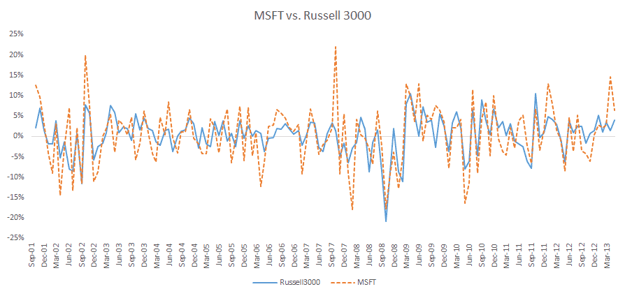
Let’s plot the monthly excess returns of Microsoft and Russell 3000 (market proxy):
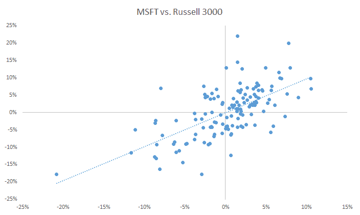
Next, we plot the scatter plot for the two data sets and draw a linear trend line to outline the correlation between the two:
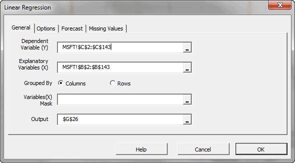
Using the linear regression wizard in NumXL, designate the monthly excess returns of Microsoft as the dependent variable (Y) and those of Russell 3000 as the independent variable (i.e. X).
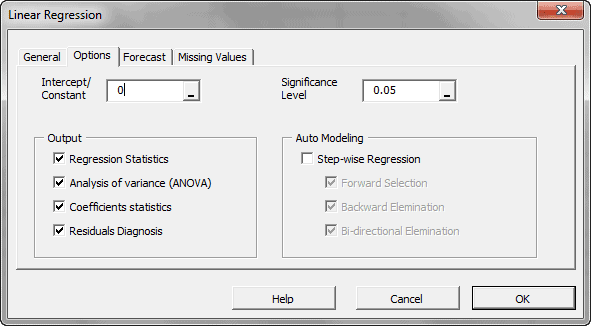
From the “Options” tab in the regression dialog box, set the intercept/constant value to zero.
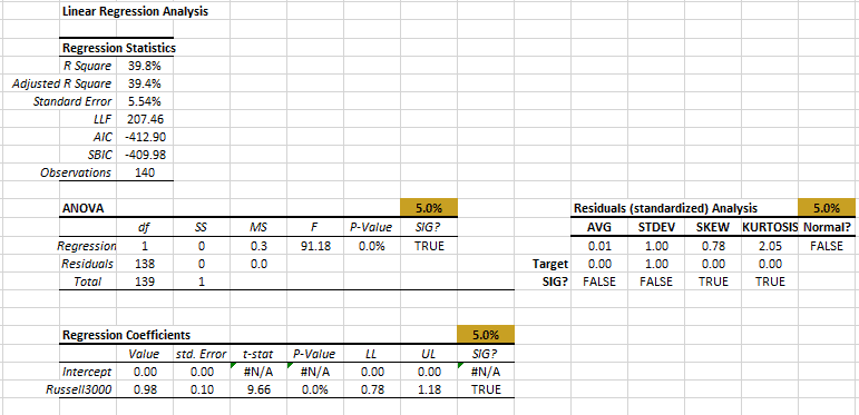
The regression model (i.e. CAPM) is statistically significant (ANOVA table) and captures about 40% of MSFT monthly excess return variance. The Beta (i.e. Russell 3000 coefficient) has an average value of 0.98 with an error of 0.10.
This is good so far, so let’s examine the standardized residuals of the regression (right-most table). The residuals exhibit a positive skew and fat tails, and thus it fails the normality test.
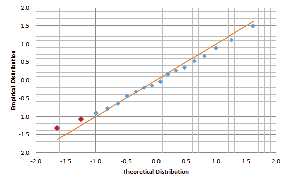
To get a better idea about the residuals distribution, we create the QQ plot with a Gaussian theoretical distribution:
The QQ-Plot shows a small deviation from normality at positive values (i.e. skew) and a fat left tail (negative).
Before we start using the CAPM and our regression beta to determine the appropriate required return of Microsoft, we should ask ourselves a key few questions first:
Is the regression model stable? Does the Beta’s value significantly differ throughout the sample data?
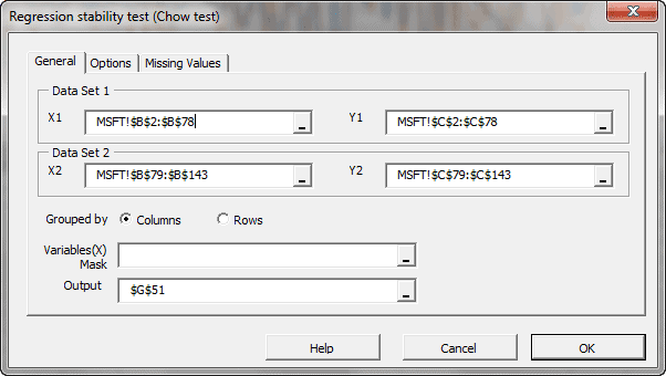
A: To answer this question, let’s divide the sample data into two subsets: data set 1 includes all observations prior to 2008 (~ 70 observations) and data set 2 covers observations starting from January 2008 to May 2013 (~ 70 observations).
Using the Regression Stability Test Wizard in NumXL, we conduct this imperative test. Similar to what we did with the regression wizard, the Russell’s excess returns are the independent (X) variable, and the MSFT returns are the dependent variable (Y).
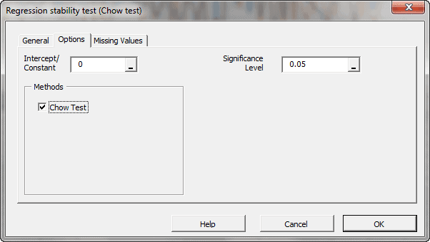
In the “Options” tab, set the intercept/constant to zero.
Now, Click “OK.” The Wizard generates the statistical stability test output table.
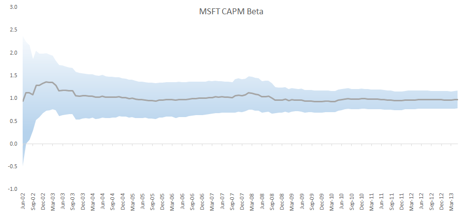
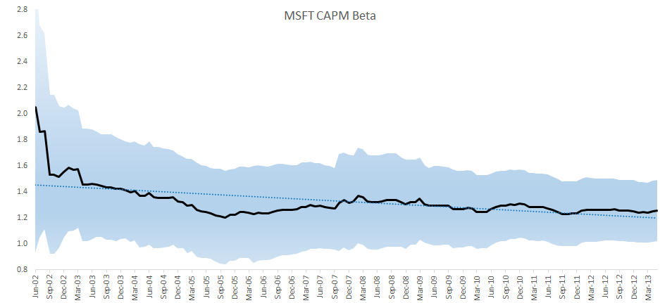
The Beta value is stable throughout our sample data set (2001 to 2013). Let’s compute and plot the beta value throughout the data set. The shaded area is our 95% confidence interval.
Are the regression’s standardized residuals serially (aka auto) correlated?
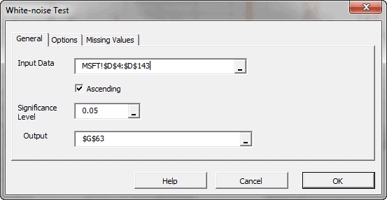
A: The white noise test answers this specific question, and is available in the NumXL statistical tests tab.
In the “Options” tab, set the maximum lag order to 12 (1 year). Click “OK.”
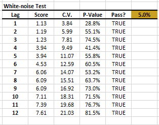
The residual’s time series exhibits no significant serial correlation.
So far, we found the following:
- The monthly returns of Microsoft stock have an average sensitivity of 0.98 with the overall market.
- The residual (aka idiosyncratic) risk (i.e. σεσε ) is around 5.54%.
Q: Do we have observation(s) that significantly affect the regression more than others (i.e. Influential data)?
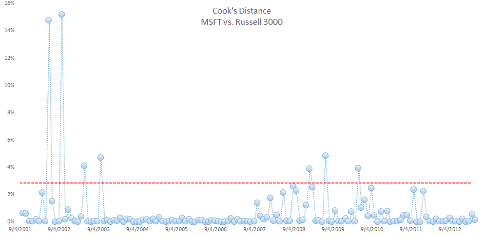
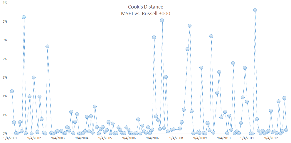
To answer the question above, we compute the Cook’s distance for each observation in the sample data. Furthermore, we use the heuristic threshold of $\frac{4}{N}$ to identify those influential points. N is the number of non-missing values in the data set.
To handle influential an data point, we decided to remove it by setting the MSFT returns to #N/A, thus removing the observation from any analysis. We remove one observation (the one with the highest Cook’s distance) at a time, then recalculate the Cook’s distance for the remaining data points using the reduced data set. Note that the threshold slightly increases as we drop observations. We continue with the process until no apparent influential data is in sight.
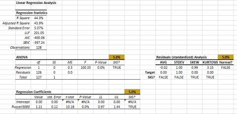
Note that the $\frac{4}{N}$ threshold is a heuristic, so we accepted data points whose Cook’s distance is slightly higher than the threshold. Recalculating the regression (SHIFT+F9), we observe the new Beta value (1.21) and regression error (5.07%).
Plotting the CAPM Beta value throughout the sample data, we observe that the Beta slightly changes over time and is trending lower over time. One may conclude that MSFT’s sensitivity to market risk is going down, due to its market-cap or the nature of investment that the company itself is undertaking.
Case 2: IBM
International Business Machines (IBM) Corporation provides information technology (IT) products and services worldwide. The company operates in five segments: Global Technology Services, Global Business Services, Software, Systems and Technology, and Global Financing. IBM is publicly traded, listed on NYSE with a market cap of 233B.
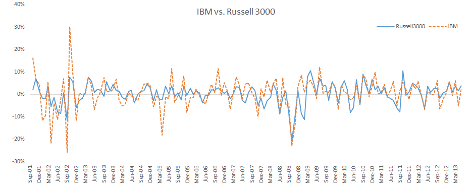
Let’s plot the IBM monthly excess returns along with the Russell 3000 (market proxy) excess returns.
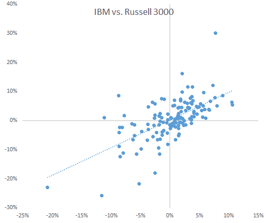
Next, we plot the scatter plot for the two data sets and draw a linear trend line to outline the correlation between the two.
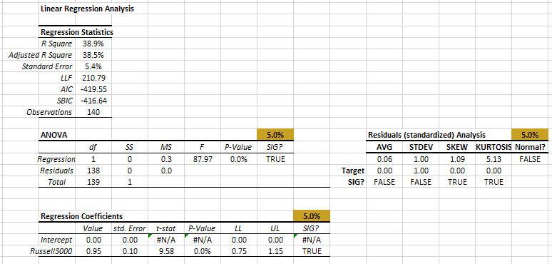
The two series demonstrate a strong correlation between them. Again, using the Regression Wizard, designate IBM excess returns as the dependent variable and the Russell 3000 as the independent, setting the intercept/constant to zero.
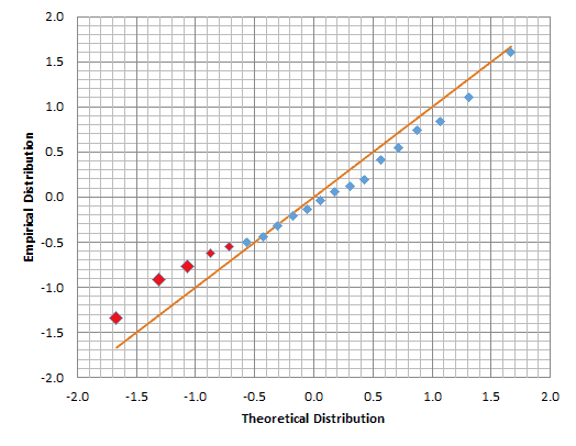
The output tables show similar results to what we saw with the Microsoft case. Let’s examine the residuals distribution closer using the QQ-Plot.
The QQ-plot exhibits positive skew, with a heavy fat tail on the left (negative) side.
Before we start using the CAPM and our regression beta to determine the appropriate required return of Microsoft, we ought to ask ourselves a key few questions:
Q: Is the regression model stable? Does the Beta’s value significantly differ throughout the sample data?
Again, we’ll divide the data set into 2 separate sub-sets: data set 1 includes all observations prior to 2008, and data set 2 includes all observations starting from January 2008 to date. Using the NumXL regression stability test, we specify the independent (X) and dependent variable (Y) values for each data set, set the intercept to zero, and click “OK.”
The test failed! We have a structural break in the data set. This can be interpreted as the Beta value changed significantly.
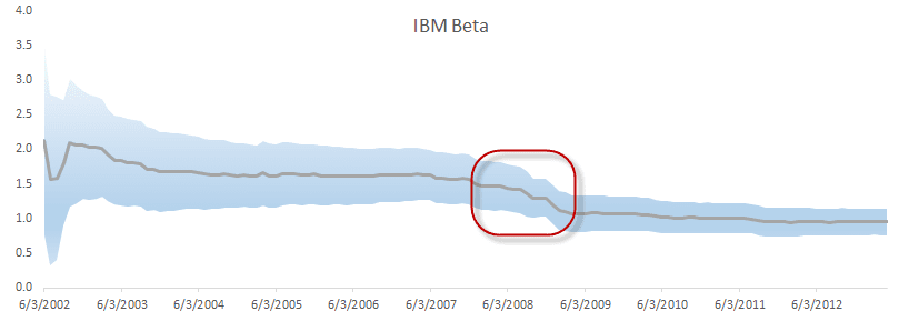
What can we do now? Let’s first plot the Beta value over time in an attempt to identify the point(s) where structural change commenced.
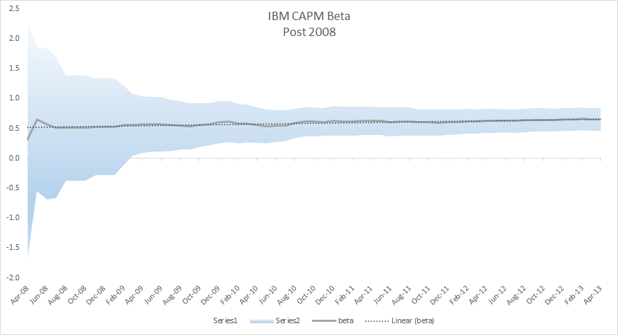
The IBM stock has undergone a Beta starting in 2008. This can be due to internal company policy change: type of investment, particular market exposure, etc. The important fact here is that the identity of the IBM stock morphed (with respect to CAPM).
In sum, we need to toss away the observations prior to 2008 and use the later observations (i.e. 2008 to May 2013) to estimate the CAPM Beta.
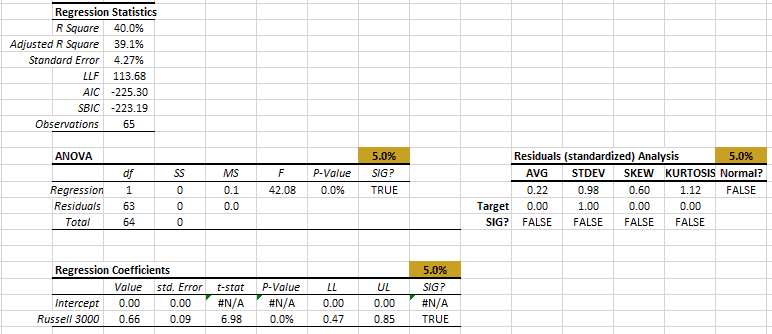
Examining the regression outputs (using post-2008 observations), the Beta has a mean value of 0.66. Furthermore, the residual diagnosis tests all passed. Additionally, the non-systematic risk (i.e. regression standard error) is around 4%.
In short, the IBM stock morphed from being a high beta value above 1 to a value lower than one.
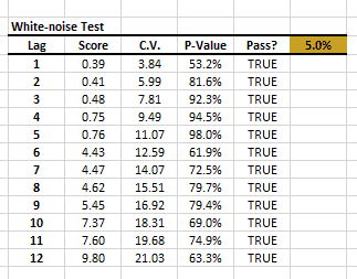
Q: Are the regression’s standardized residuals serially (aka auto) correlated?
A: The white noise test answers this specific question, and is available in NumXL’s statistical tests tab.
The residual’s time series exhibits no significant serial correlation.
Q: Do we have observation(s) that significantly affect the regression more than others (i.e. influential data)?
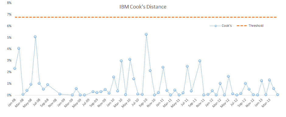
To answer the question above, we compute the Cook’s distance for each observation in the sample data post-2008.
Similar to what we did in the Microsoft case, we removed influential data by setting the MSFT returns to #N/A, thus removing the observation from any analysis. We remove one observation (one with the highest cook’s distance) at a time, then recalculate the Cook’s distance for the remaining data points using the reduced data set. Note that threshold slightly increases as we drop observations. We continue with the process, until no apparent influential data is in sight.
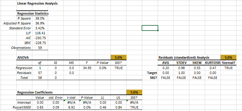
Recalculating the regression model:
The non-systematic error dropped to 3.42% (from 4.27% earlier), and all the residuals diagnosis tests are passed.
Plotting the CAPM beta value throughout the sample data, we observe that the Beta slightly changes over time and is trending upward over time. One may conclude that MSFT’s sensitivity to market risk is going up, due to the nature of new investment that the company is undertaking.
Conclusion
In this paper, we demonstrated the process for computing the CAPM Beta for two tech stock: IBM and MSFT.
In both cases, we proposed a simple linear regression model for the stock’s monthly excess returns versus the monthly excess returns of the Russell 3000 Index (market proxy). The regression slope is the empirical CAPM Beta and the regression standard error is viewed as the stock’s non-systematic (idiosyncratic) error.
Afterward, we carried on a plain regression analysis process: ANOVA, coefficient’s value test, residuals diagnosis, regression stability test, and influential data analysis.
The computed CAPM Beta significantly improved as we carried our thorough analysis to the regression results.
All tools you need to carry on this exercise are part of NumXL 1.60 Pro. The CAPM is a relatively simple one-factor model. In later issues, we’ll tackle multi-factors (e.g. Fama-French three (3) factor model (FFM), etc.), which may add some numerical complexity while the basic steps and intuition remain the same.


