Theoretically, crude oil future prices reflect the market participants’ expectation of future demand and supply, as well as their overall uncertainty.
The crude oil future market is an interesting market to analyze. Laws of cost-of-carry, supply, and demand still apply, but geopolitical risk weighs on relative prices.
Historically, the oil futures curve is often found in backwardation, which means higher prices for short-term contracts than for long-term contracts. This is often explained by a theoretical term called “convenience yield.” Convenience yield is conceptually similar to dividends in equity, where it favors physical possession of the stock over future delivery due to the dividend cash payments. In the crude oil market, convenience yield may signal market worry on future oil supply (or delivery), due to some geopolitical concerns and the tendency to favor holding the commodity now.
In this white paper, we will not delve into the theoretical economics behind the price changes or their spreads. Instead, we will examine the daily prices of the first four (4) contracts of WTI CL futures listed on NYMEX. Next, using exchange rules for WTI/CL contract trading, we will compute the number of days to the delivery month for each contract to construct the futures curve. Finally, we will carry out principal component analysis (PCA) in an attempt to uncover the core drivers behind the futures curve changes (i.e. level and general shape).
Why should we care?
The oil future market is very complex in its design, and, in this paper, we will attempt to uncover and simplify the underlying drivers reflected in the daily relative prices of different contracts for a better understanding and better hedging for a portfolio of such instruments.
Background
The general demand for petroleum products is highly seasonal and is greatest during the winter months, when countries in the Northern Hemisphere increase their use of distilled heating oils and residual fuels. Supply of crude oil, including both production and net imports, also shows a similar seasonal variation but with a smaller magnitude.
During the summer months, supply exceeds demand and petroleum inventories normally build; whereas during the winter, demand exceeds supply and inventories are drawn down. As a result, inventories also demonstrate seasonality.
In theory, futures prices are computed as follows:
$$F_{t,T}=s_t\times e^{(r_{t,T}+x_{t,T}-q_{t,T})(T-t)}$$
Where
- $F_{t,T}$= future prices at time ($t$) for delivery at $T$.
- $S_t$ = WTI spot prices for delivery at Cushing, OK
- $t$ = time now
- $T$ = future delivery time
- $r_{t,T}$ = nominal (per annum) interest rate at time ($t$) for maturity $T$
- $x_{t,T}$ = nominal (per annum) marginal storage cost at time ($t$) for delivery $T$.
- $q_{t,T}$ = nominal (per annum) theoretical convenience yield at time ($t$) for delivery $T$
Now, let’s take the logarithm of each side:
$$\ln(F_{t,T}) = \ln(S_t) + (r_{t,T}+x_{t,T}-q_{t,T})(T-t) $$
To carry out our analysis, we will use the logarithm of future prices and include the log of the WTI spot prices into the data set.
Next, we will compute the net of the interest rate, storage and convenience yield rates (i.e. $\phi_{t,T}$ ), which can be expressed as follows:
$$\phi_{t,T} = r_{t,T}+x_{t,T}-q_{t,T} = \frac{\ln(F_{t,T}/S_t)}{T-t}$$
Note that $\phi_{t,T}$ theoretically consists of three loosely correlated factors (interest, storage and convenience annual yield), so we’d expect that applying a PCA-type of analysis should yield no more than three (3) factors.
Data Preparation
In this paper, we will use the closing marks of the immediate four (4) traded NYMEX CL future contracts of the EIA web site. Furthermore, we also use the spot prices for WTI crude oil at Cushing, OK (delivery location for NYMEX CL contracts) of the EIA website as well.
To compile our data set, we use the number of days to the 1st day of the delivery month as our horizon (i.e. the independent variable of the future curve). We refer to this as days-to-delivery or DTD.
Next, according to NYMEX product specification, the trading of a crude oil future contract terminates base on the following rule(s):
“Trading in the current delivery month shall cease on the third business day prior to the twenty-fifth calendar day of the month proceeding the delivery month. If the twenty-fifth calendar day of the month is a non-business day, trading shall cease on the third business day prior to the last business day proceeding the twenty-fifth calendar day. In the event that the official Exchange holiday schedule changes subsequent to the listing of Crude Oil futures, the originally listed expiration date shall remain in effect. In the event that the originally listed expiration day is declared a holiday, expiration will move to the business day immediately prior”
Using the last trading day rules, we determine when the front contract switches to the following month contract, and, thus, compute the proper trading days to the 1st day of the delivery month. For computing the trading days, adjusting for weekends and holidays, we used the NumXL calendar functions with the USD calendar.
As a result, for each trading day, we use the four (4) contracts to construct a future curve (future prices versus number of days to deliver (DTD)).
Next, on each day, using the future curve above, we interpolate/extrapolate (cubic spline) the future prices for delivery terms ranging from 10 days to 120 days (12 terms).
Next, using the formula below, we transform the future prices into the net of the interest rate, storage cost and convenience yield (i.e. $\phi_{t,T}$)
$$\phi_{t,T} = r_{t,T}+x_{t,T}-q_{t,T} = \frac{\ln(F_{t,T}/S_t)}{T-t}$$
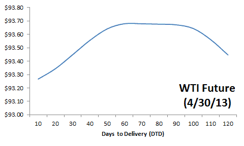
For example, on April 29, 2013, the WTI future curve exhibits a hump-shaped curve:
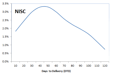
On the same day, the implied (computed) net interest rate, storage and convenience yield (NISC) for each delivery term, the $\phi_{t,T}$ exhibits the following shape (graph below).
Although the future prices between 50-100 DTD remains flat, the underlying net of interest, storage and convenience yield changes due to the change in time-to-delivery.
Finally, we compute twelve (12) time series for the net interest, storage and convenience yield (NISC) for delivery terms ranging from 10 to 120 days.
Analysis
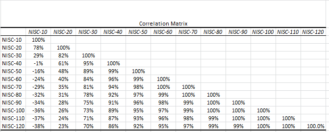
Let’s first examine the correlation between the twelve NISC input time series.
The short-term deliveries (< 30 days) of the NISC correlate weakly with longer-terms futures. Note that this phenomenon is not found in the raw future prices.
Now, let’s run PCA analysis. Before we launch the wizard, insert a row above the input data for the mask variable and set all its values to 1. This will help us to exclude input variables without re-doing the analysis.
Launch the PCA Wizard, specify input variables and compute the PCA statistics.
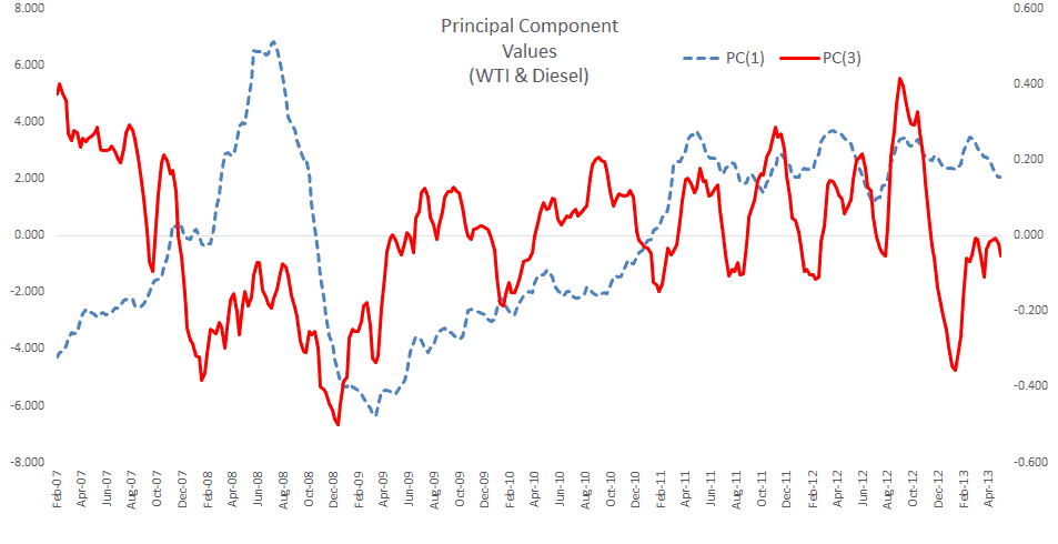
PCA shows that the first two principal components (aka drivers) account for 98.7% of the overall variation, and the first three principal components capture 99.9%.
Let’s examine the loadings of those drivers in an attempt to find a practical/physical proxy for them. For the first principal component:
The first PC loadings (aka term structure) exhibit a pattern similar to the yield curve: Contago in short term, and flat for longer-term. We may think of the first component as a proxy for the interest rate.
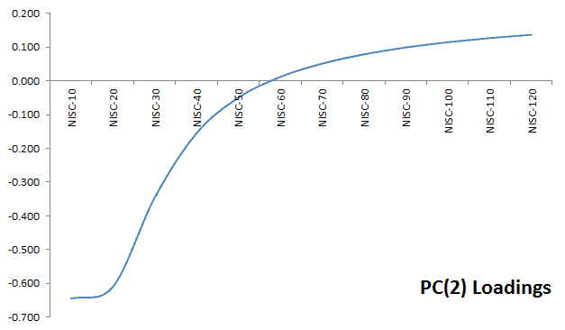
The second principal component’s (aka driver) loading exhibits the following pattern:
This pattern is similar to the PC1, with the exception of the kink for 10-20 days, and the negative values up to 50 days. This may be assumed as a proxy for the convenience yield; short-term tenors have negative values causing the future prices to rise and possibly creating a backwardation. For longer-term tenors, the value is positive, reducing the future price and strengthening the backwardation.
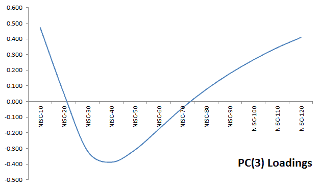
The third principal component is relatively harder to explain:
Can this be the storage cost per year? Unlikely, as the loading goes negative between 20 and 70 days to delivery. Fortunately, its variance and contribution to the overall variation are relatively small.
Conclusion
In sum, we found that the net interest, storage and convenience yield (NISC) of WTI futures are primarily driven by two uncorrelated drivers. The first driver exhibits a term structure similar to the yield curve and the second driver was hypothesized as a proxy to the convenience yield.
Wait a minute!
You may wonder: can I leverage a interest rate instrument (e.g. Eurodollar, swaps, etc.) to hedge the interest rate exposure in my WTI futures portfolio?
In a follow up paper, we will examine the LIBOR yield curve data into our analysis and fine tune our risk dirvers further, isolating the storage and convenience yield from the interest rate.
Why do we care?
A portfolio of WTI future contracts can be hedged (97.8% effective) for non-spot price changes using only two (2) different future contracts.
- What about spot changes?
- What is the hedging ration?
- How often do we re-balance the hedge?
In a follow-up paper, we’ll discuss the hedging in relation to PCA in further details.
Why do we stop here?
There is a lot of material here to swallow, so we opted to pause at this stage to give you opportunity to digest and get comfortable with our earlier discussion, and better prepare you for a more advanced handling of the topic.

