Weighted Moving Average (WMA) – Smoothing
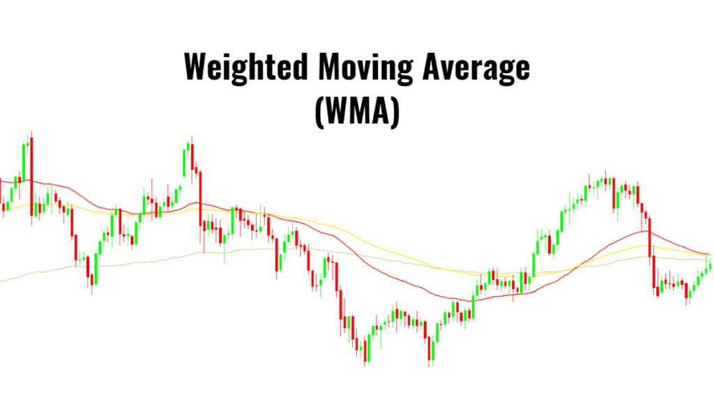
A moving average is commonly used with time-series data to smooth out short-term fluctuations and highlight longer-term trends or cycles. A weighted moving average has multiplying factors to give different weights to data at different positions in the sample window.
$$Y_t=\frac{\sum_{i=1}^N{W_i X_{t-i}}}{\sum_{i=1}^N W_i}$$
- $W_i$ is the i-th position weight-factor
- $\{X_t\}$ is the original time series
- $\{Y_t\}$ is the smoothed time series
- $Y_t$ uses the prior N-values of $X_t$ observations (i.e. $\{X_{t-1},X_{t-2},\cdots ,X_{t-N}\}$)
The weighted moving average has a fixed window (i.e., N), and the factors are typically chosen to give more weight to recent observations.
The window size (N) determines the number of points averaged at each time, so a larger windows size is less responsive to new changes in the original time series, and a small window size can cause the smoothed output to be noisy.
For out of sample forecasting purposes:
- $\{w_i\}$ is the normalized weight-factors
Example 1 :
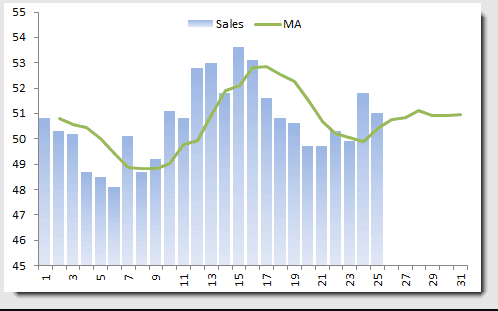
Let’s consider monthly sales for Company X, using a 4-month (equal-weighted) moving average.
Note that the moving average always lags behind the data, and the out-of-sample forecast converges to a constant value.
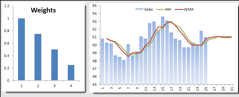
Let’s try to use a weighting scheme (see below) that emphasizes the latest observation.
We plotted the equal-weighted moving average and WMA on the same graph. The WMA seems more responsive to recent changes, and the out-of-sample forecast converges to the same value as the moving average.
Example 2:
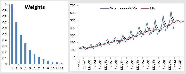
Let’s examine the WMA in the presence of trend and seasonality. For this example, we’ll use the international passenger airline data. The moving average window is 12 months.
The MA and the WMA keep pace with the trend, but the out-of-sample forecast flattens. Furthermore, although the WMA exhibits some seasonality, it is always lagging behind the original data.
Tutorial Video
Files Examples
Please click the button below to download Weighted Moving Average example.


