In this issue, we will tackle the probability distribution inference for a random variable.
Why do we care? As a start, no matter how good a stochastic model you have, you will always end up with an error term (aka shock or innovation) and the uncertainty (e.g. risk, forecast error) of the model is solely determined by this random variable. Second, uncertainty is commonly expressed as a probability distribution, so there is no escape!
One of the main problems in practical applications is that the needed probability distribution is usually not readily available. This distribution must be derived from other existing information (e.g. sample data).
What we mean by probability distribution analysis is essentially the selection process of a distribution function (parametric or non-parametric).
In this paper, we’ll start with the non-parametric distributions functions: (1) empirical (cumulative) density function and (2) the Excel histogram. In a later issue, we’ll also go over the kernel density function (KDE).
Background
1.Empirical Density Function (EDF)
The empirical distribution function (EDF), or empirical cdf is a step function that jumps by 1/N at the occurrence of each observation.
Where:
- $I\{A\}$ is the indicator of an event function
- $I\{x_i \leqslant x\}=\begin{cases} 1 & \text{ if } x_i \leqslant x \\ 0 & \text{ if } x_i > x \end{cases}$
The EDF estimates the true underlying cumulative density function of the points in the sample; it is virtually guaranteed to converge to the true distribution as the sample size gets sufficiently large
To obtain the probability density function (PDF), one needs to take the derivative of the CDF, but the EDF is a step function and differentiation is a noise-amplifying operation. As a result, the consequent PDF is very jagged and needs considerable smoothing for many areas of application.
2. Histograms
In statistics, a histogram is a graphical representation showing a visual impression of the distribution of data. Histograms are used to plot the density of data, and often for density estimation, or estimating the probability density function of the underlying variable.
In mathematical terms, a histogram is a function mi that counts the number of observations whose values fall into one of the disjoint intervals (aka bins).
$$N=\sum_{i=1}^k m_i$$
Where:
- $N$ is the total number of observations in the sample data
- $k$ is the number of bins
- $m_i$ is the histogram value for the i-th bin
And a cumulative histogram is defined as follows:
The frequency function $f_i$ (aka relative histogram) is computed simply by dividing the histogram value by the total number of observations;
One of the major drawbacks of the histogram is that its construction requires an arbitrary assignment of bar width (or bins number) and bar positions, which means that unless one has access to a very large amount of data, the shape of the distribution function varies heavily as the bar width (or bin number) and positions are altered.
Furthermore, for large sample size, the outliers are difficult or perhaps impossible to see in the histogram, except when they cause the x-axis to expand.
Having said that, there are a few methods for inferring the number of histogram bins, but care must be taken to understand the assumptions made behind their formulation.
Sturges’ formula
The Sturges’ method assumes the sample data follow an approximate normal distribution (i.e. bell shape).
Furthermore, for large sample size, the outliers are difficult or perhaps impossible to see in the histogram, except when they cause the x-axis to expand.
$$k=\left \lceil \log_2 N +1 \right \rceil$$
Where:
- $\left \lceil X \right \rceil$ is the ceiling operator
Square root formula
This method is used by Excel and other statistical packages. It does not assume any shape of the distribution:
$$k= \sqrt {N}$$
Scott’s (normal reference) choice
Scott’s choice is optimal for random sample of normal distribution:
$$k=\frac{3.5\hat\sigma}{\sqrt[3]{N}}$$
Where:
- $\sigma$ is the estimated sample standard deviation
Freedman-Diaconis’s choice
$$h=2\frac{\mathrm{IQR}}{\sqrt[3]{N}}$$
Where:
- $h$ is the bin size
- $\mathrm{IQR}$ is the inter-quartile range
$$k=\left \lceil \frac{x_{\mathrm{max}}-x_{\mathrm{min}}}{h} \right \rceil$$
Decision based on minimization of risk function ($L^2$)
$$\mathrm{min}\{L^2\}=\mathrm{min} \left ( \frac{2\bar m-v}{h^2} \right )$$
Where:
$$\bar m = \frac{\sum_{i=1}^k m_i}{k}=\frac{N}{k}$$ $$v=\frac{\sum_{i=1}^k (m_i – {\bar m}^2)}{k}=\frac{1}{k}\sum_{i=1}^k m_i^2-\frac{N^2}{k^2}$$
$$\mathrm{min}\{L^2\}=\mathrm{min} \left ( \frac{2\bar m-v}{h^2} \right )$$
3.Kernel Density Estimate (KDE)
An alternative to the Excel histogram is kernel density estimation (KDE), which uses a kernel to smooth samples. This will construct a smooth probability density function, which will in general more accurately reflect the underlying variable. We mentioned the KDE for sake of completion, but we will postpone its discussion to a later issue.
EUR/USD Returns Application
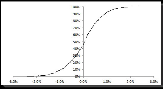
Let’s consider the daily log returns of the EUR/USD exchange rate sample data. In our earlier analysis (ref: NumXL Tips and Hints – Price this), the data was shown to be a Gaussian white noise distribution. The EDF function for those returns (n=498) is shown below:
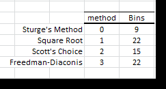
For an Excel histogram, we calculated the number of bins using the 4 methods
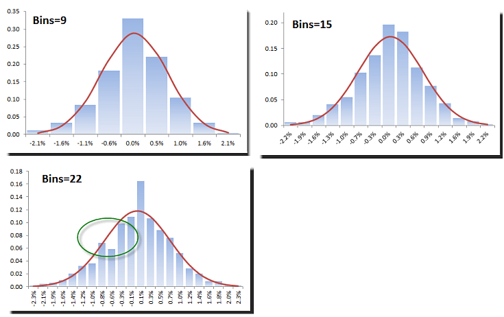
Next, we plot the relative Excel histogram using those different bins numbers. We overlay the normal probability density function (red-curve) for comparison
Although we have a relatively large data set (n=498) and the EDF and statistical test exhibit Gaussian distributed data, the selection of different bin sizes can distort the density function.
Scott’s choice (n=15) describes the density function best, and next would be Sturge’s.
Conclusion
In this issue, we attempted to derive an approximate of the underlying density probability using a sample data Excel histogram and the (cumulative) empirical density function.
Although the data sample is relatively large (n=498), the Excel histogram is still a fairly crude approximation and very sensitive to the number of bins used.
Using the rules of thump (e.g. Sturge’s rule, Scott’s choice, etc.) can improve the process of finding better bins number, but they make their own assumptions about the shape of the distribution and an experienced (manual) examination (or eyeballing) is needed to ensure proper Excel histogram generation.


